Technical Note 1: Seamless workflow for defining archaeological site densities with contour lines by using the open source (geo-)statistical language R

Ahlrichs, Jan Johannes^1,2, Henkner, Jessica^1,4 and Schmidt, Karsten^1,3,4

¹ Collaborative Research Center 1070 ResourceCultures, University of Tübingen

² Institute of Pre- and Protohistory and Medieval Archaeology, University of Tübingen

³ eScience-Center, University of Tübingen

⁴ Department of Geosciences, Soil Science & Geomorphology, University of Tübingen

The entire script with short description is attached for download. Additionally, we provide a test dataset, which we have used for further testings. The test dataset contains a complete random selection of burial sites from the Hallstatt period in Baden-Württemberg after Paret (1961).
This technical section is made to evolve! Please share your thoughts, requirements and suggestions regarding the described issues to

Jan Ahlrichs jan.ahlrichsspam prevention@uni-tuebingen.de and
Karsten Schmidt karsten.schmidtspam prevention@uni-tuebingen.de
 

Download: R-Script

Download: Description (PDF)

Download: Test materials

Description

The development and analysis of distribution maps is one of the most frequent applications in archaeological research. For instance, sets of archaeological sites can be used to calculate larger areas, which represent, for example, the spatial spread of a culture or the site density within an area of interest. In many previous studies this is archived manually. However, this process is problematic because it is based on a subjective impression which most likely leads to many different results and interpretations. In contrast, a standardized workflow as well as standardized settings and parameters enable the possibility to share the results and make them comparable to other similar processed geo data.

Besides reducing the personal influence of different experts, computer generated maps facilitate the description of archaeological phenomena on a large scale and/or high resolution. Here we present a semi-automated workflow, which was developed in the open source statistical language R, by using different state-of-the-art packages to facilitate each single methodological step in one seamless workflow. This open source script represents a time- and cost-efficient solution, which simplifies otherwise complicated workflows and/or expensive software solutions and calculates reproducible maps with isolines. Therefore it allows researchers an objective interregional and chronological comparison by using the standardized workflow to generate the density maps and/or different times, e.g. different time periods on the same regional extend, and/or different regions and the development over time.

In German prehistoric archaeology contour lines or isolines are being used to describe archaeological site densities since the early 1990s (Zimmermann 1992; Saile 1998: 139). Originally for archaeological research, this method was introduced by Mats P. Malmer in the late 1950s (Malmer 1957; Malmer 1962: 697–702; Sørensen 2002: 170–171).

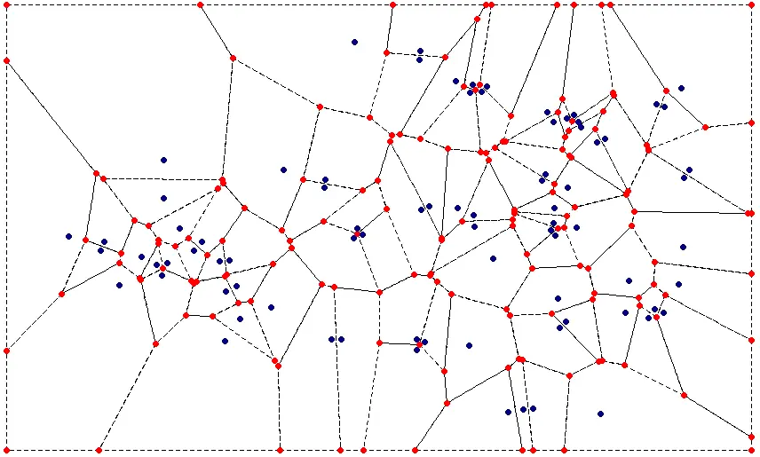
The computation of these isolines is done in several steps, the basic principle didn’t change much. First of all a set of archaeological sites with distinct coordinates is needed. On the basis of these sites so-called Thiessen polygons or Voronoi diagrams are calculated. The nodes of these polygons are defined by the perpendicular bisectors of Delaunay triangulations – this process is also called tessellation (Zimmermann 1992). Liebling and Pournin (2012) are providing a good review about the methodological and historical developments of the Voronoi diagrams ranging back to Kepler and Descartes. The calculation of the distance between the archaeological sites and the nodes of the Thiessen polygons is based on the principle of the largest empty circle – LEC (Toussaint 1983; Preparata and Shamos 1988: 255–262). The distance of a node to the nearest three sites corresponds to the radius of a circle in which there are no further sites (Zimmermann et al. 2004: Fig. 4).

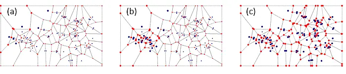
Consequently, in regions with a high density of archaeological sites, there are several small empty circles. On the other hand, regions with a very low density of archaeological sites are defined by few empty circles with larger radii. Based on the distances from the Thiessen polygons' nodes to the nearest archaeological sites a geostatistical interpolation approach can be used to estimate a distance map on a predefined resolution. Common approaches are Inverse-Distance Weighted, Spline Interpolation and Kriging. We used one standard version of Kriging so called Ordinary Kriging to compute the distances between the archaeological sites. Kriging originates from the mining industry and is based on the idea of a mining engineer D.G. Krige and a statistician H.S. Sichel (Conolly and Lake 2006: 97–101; Hengl 2011). The statistical formulation is based on the work of the mathematician G. Matheron (Cressie 1993; Webster and Oliver 2001). Ordinary Kriging represents the most common Kriging method and is based on the following assumptions (Cressie 1993):

(i) Global, constant mean of the random function is unknown.

(ii) The random function is assumed to be at least intrinsic stationary with a known variogram function.

The following equations and descriptions are based on Hengl (2011)

(1)

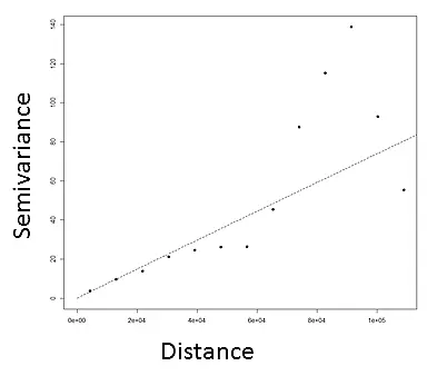
where µ is the global mean and ε′ (x) is the spatially correlated stochastic part of variation. The variogram function is derived by the analysis of point data and the plotting of the so-called semivariances ( Hengl 2011):

(2)

where z (x_i) is a value of an known sample location and z (x_i + h) is the value of a neighbor at distinct distance h.

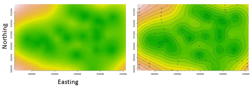
Finally lines of constant values (contour or isolines) are delineated from the krigged distance map to describe the relative density of the archaeological sites. As aforementioned these isolines can be used for the description and comparison of distributions maps of archaeological cultures (Saile 1998: 139–177; Saile 2003; Zimmermann et al. 2004; Zimmermann et al. 2009; Wendt et al. 2010). Additionally, they can be used in order to model territories of collectors, i.e. to illustrate the state of research (Frank 2007; Mischka 2007: 230–232; Pankau 2007: 102–112) and to analyze the distribution of archaeological finds within an excavated area (Loew 2006). If you are interested in doing the latter with our script, please make sure to adjust the cell size and the unit of the contour line delineation.

Based on the mathematical assumptions only euclidean distances between sites are used for computation, therefore geographical features like rivers or mountains influencing the possible density representation (e.g. Perceived distance – Perception) etc. are not taken into account. If you would like to use e.g. terrain information to guide the Kriging estimates you can adjust the script by using e.g. ‘Universal Kriging’ instead. Furthermore the isoline dataset depends on a distinct point dataset, as soon as archaeological sites are being removed or added, the results can change and different isolines and site densities are generated (Ducke and Kroefges 2008; Mischka 2009: 50).

Different R packages are necessary for each single step to delineate archaeological site density. A brief introduction to each package is given in table 1.

Tab 1. R packages used for the delineation of archaeological site density

All libraries have to be installed on a local machine and implemented via library command.

- #R-SCRIPT Part 1 – Libraries

[1] library("sp")

[2] library("deldir")

[3] library("ggplot2")

[4] library("rgeos")

[5] library("geoR")

[6] library("maptools")

[7] library("rgdal")

To implement the Voronoi polygon tessellation of a point layer, we used the ‘voronoipolygon’ function from C. Farmer (http://carsonfarmer.com/2009/09/voronoi-polygons-with-r/).

Some general setting related to working directory, Spatial point dataset of the archaeological sites, Layer, Resolution of the final raster dataset, and Elevation bands. [important remark: Set the correkt Working Directory which contains and stores all your relevant data].

Load and prepare the spatial point dataset including exclusion of duplicates.

Calculate all distances between Voronoi polygon nodes and archaeological sites.

Generate the final raster dataset based on a given cell size and a rectangular shape defined by the minimum and maximum coordinate of the spatial point dataset including a small buffer defined by the cell size.

Bivand, R.S., Keitt, T., Rowlingson, B. (2015). Bindings for the Geospatial Data Abstraction Library. R-package ‘rgdal’, http://www.gdal.org, https://r-forge.r-project.org/projects/rgdal/.

Bivand, R.S. and Lewin-Koh, N. (2016). Tools for Reading and Handling Spatial Objects. R-package ‘maptools’, r-forge.r-project.org/projects/maptools/.

Bivand, R.S., Rundel, C. (2016). Interface to Geometry Engine – Open Source (GEOS). R-package ‘rgeos’, https://r-forge.r-project.org/projects/rgeos/ http://trac.osgeo.org/geos/.

Conolly, J. and Lake, M. (2006). Geographical Information Systems in Archaeology. Cambridge: Cambridge University Press.

Cressie, N.A.C. (1993). Statistics for Spatial Data, revised edition. John Wiley and Sons, New York, p. 416.

Ducke, B. and Kroefges, P. C. (2008). From Points to Areas: Constructing Territories from Archaeological Site Patterns Using an Enhanced Xtent Model. In: A. Posluschny, K. Lambers and I. Herzog (eds.), Layers of Perception. Proceedings of the 35th International Conference on Computer Applications and Quantitative Methods in Archaeology (CAA), Berlin, Germany, April 2–6, 2007. Kolloquien zur Vor- und Frühgeschichte 10. Bonn: R. Habelt, pp. 245–251.

Frank, T. (2007). Zur Bedeutung der Tätigkeit von Sammlern für die Archäologie. Die Kunde N. F., 58(1), pp. 91–106.

Hengl, T. (2011). A Practical Guide to Geostatistical Mapping. 2. Edition, University of Amsterdam, 291p.

Liebling, T.M. and Pournin, L. (2012). Voronoi Diagrams and Delaunay Triangulations: Ubiquitous Siamese Twins. Documenta Maethematica, Extra Volume ISMP, pp. 419–431.

Loew, S. (2006). Rüsselsheim 122 und die Federmessergruppen am Unteren Main. PhD. Universität zu Köln.

Malmer, M. P. (1957). Pleionbegreppets betydelse för studiet av förhistoriska innovationsförlopp. Svenska Fornminnesföreningens tidskrift, 58(1), pp. 160–184.

Malmer, M. P. (1962). Jungneolithische Studien. Acta Archaeologica Lundensia 8/2. Lund: Gleerups.

Mischka, D. (2007). Methodische Aspekte zur Rekonstruktion prähistorischer Siedlungen. Landschaftsgenese vom Ende des Neolithikums bis zur Eisenzeit im Gebiet des südlichen Oberrheins. Freiburger archäologische Studien 5. Freiburg: M. Leidorf.

Mischka, D. (2009). Grenzen im Neolithikum. In: S. Hesse (ed.), Grenzen in der Archäologie und Geschichte. Beiträge zur Jahrestagung der Archäologischen Kommission für Niedersachsen e.V. in Rotenburg (Wümme), 14.–16. Juni 2007. Archäologische Berichte des Landkreises Rotenburg (Wümme), 15 (1), pp. 43–65.

Pankau, C. (2007). Die Besiedlungsgeschichte des Brenz-Kocher-Tals (östliche Schwäbische Alb) vom Neolithikum bis zur Latènezeit, Volume 1. Universitätsforschungen zur prähistorischen Archäologie 142. Bonn: R. Habelt.

Paret, O. (1961). Württemberg in vor- und frühgeschichtlicher Zeit. Stuttgart: Kohlhammer.

Pebesma, E.J., R.S. Bivand, 2005. Classes and methods for spatial data in R. R News 5 (2), http://cran.r-project.org/doc/Rnews/.

Preparata, F. P. and Shamos, M. I. (1988). Computational Geometry: An introduction. New York: Springer.

Ribeiro, P.J., Diggle, P.J. (2015). Analysis of Geostatistica Data. R-packages ‘geoR’, cran.r-project.org/web/packages/geoR/.

Saile, T. (1998). Untersuchungen zur ur- und frühgeschichtlichen Besiedlung der nördlichen Wetterau. Materialien zur Vor- und Frühgeschichte von Hessen 21. Wiesbaden: Landesamt für Denkmalpflege Hessen.

Saile, T. (2003). Settlement Dynamics in the Wetterau. In: J. Kunow and J. Müller (eds.), Archäoprognose Brandenburg I. Symposium Landschaftsarchäologie und geographische Informationssysteme. Forschungen zur Archäologie im Land Brandenburg 8. Wünsdorf: Brandenburgisches Landesamt für Denkmalpflege und Archäologisches Landesmuseum, pp. 259–269.

Sørensen, M. L. S. (2002). Mats P. Malmer – An Intellectual Biography. Current Swedish Archaeology, 10(1), pp. 163–177.

Toussaint, G. T. (1983). Computing Largest Empty Circles with Location Constraints. International Journal of Computer and Information Sciences, 12(5), pp. 347–352.

Turner, R. (2015). Delaunay Triangulation and Dirichlet (Voronoi) Tessellation. R-package ‘deldir’, cran.r-project.org/web/packages/deldir/.

Wickham, W. (2009). ggplot2: Elegant Graphics for Data Analysis. Springer-Verlag New York.

Webster, R., Oliver, M. A. (2001). Geostatistics for Environmental Scientists. Statistics in Practice. Wiley, Chichester, p. 265.

Wendt, K. P., Hilpert, J. and Zimmermann, A. (2012). Landschaftsarchäologie III. Untersuchungen zur Bevölkerungsdichte der vorrömischen Eisenzeit, Merowingerzeit und der späten vorindustriellen Neuzeit an Mittel- und Niederrhein. Bericht der Römisch-Germanischen Kommission, 91(1), pp. 217–338.

Zimmermann, A. (1992). Tesselierung und Triangulation als Techniken zur Bestimmung archäologischer Funddichten. Archäologische Informationen, 15(1), pp. 107–112.

Zimmermann, A., Richter, J. Frank, T. and Wendt, K. P. (2004). Landschaftsarchäologie II – Überlegungen zu Prinzipien einer Landschaftsarchäologie. Bericht der Römisch-Germanischen Kommission, 85(1), pp. 37–96.

Zimmermann, A., Wendt, K. P., Frank, T. and Hilpert, J. (2009). Landscape Archaeology in Central Europe. Proceedings of the Prehistoric Society, 75(1), pp. 1–53.

nach oben

_{Die Bildrechte des Technical Note liegen bei Karsten Schmidt.}